Changes in accounting standards tend to be pretty dull, but this one is seismic. IFRS 9 introduces a new era for expected loss provisioning: banks now need to model expected losses throughout the lifetime of a financial instrument. In practice, this means simulating millions of realistic future scenarios in order to accurately compute probability-weighted losses. Advances in complexity science and computational economics have made this type of risk management possible, allowing financial institutions more than just simple compliance, but also true business value and competitive advantage.
If we are walking along a cliff, it is not simply enough to feel solid ground beneath our feet, it is also nice to see how far from the edge we are.
Background
IFRS 9 is a product of a number of painful lessons learned during the 2008 financial crisis, seeing its descendant IAS 39 out at the start of this year. During the financial crisis, banks recognized losses on financial assets, such as mortgages, only after they had objective evidence that the asset was impaired. This kind of provisioning was done on a so-called incurred loss basis. Even though banks knew that they were about to take significant losses, the accounting standard didn’t let them recognize them. As a result, some banks continued to pay out large dividends while the economy nose-dived.
IFRS 9 was designed to tackle exactly this issue. It introduces provisioning on an expected loss basis. On the day a financial instrument is created (for example, a mortgage is issued), the bank is now expected to hold back some provisions that take a forward-looking view of the expected future losses on that instrument. Those provisions are then updated throughout the life of the asset. Were a crisis to appear over the horizon, banks would raise provisions now — this is simply good sense. Expected loss provisioning is a bank’s way of battening down the hatches before a storm. Those provisions are set aside today with a view to smooth out the impact of future loan losses in the event of a crisis. In effect, the volatility of banks’ asset values is shifted from the balance sheet, to the income statement — protecting banks’ precious regulatory capital.
Battening down the hatches before a storm is simply good sense, why would banks not acquire the tools to do the same in the face of a crisis?
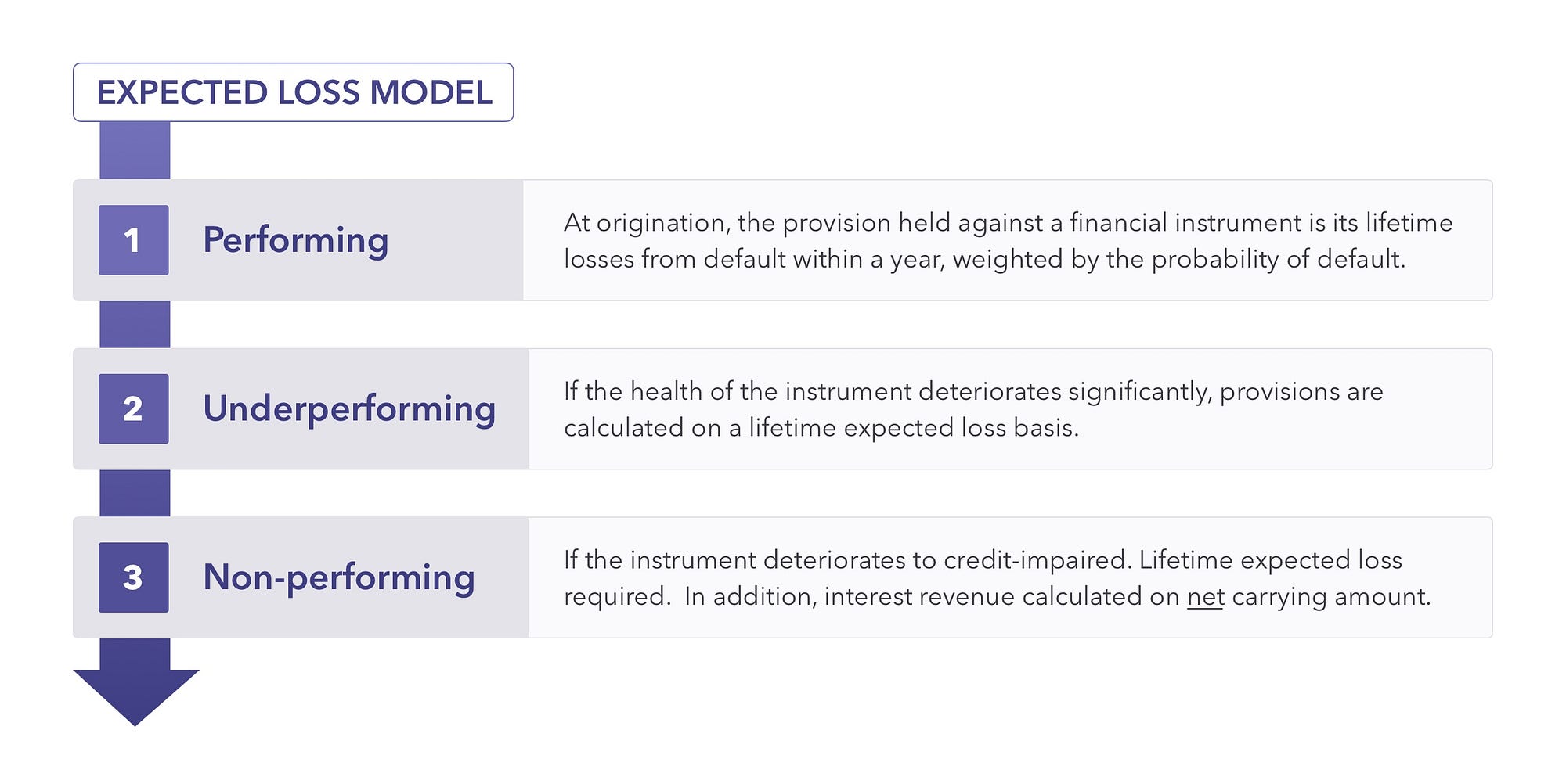
Throughout the lifetime of an asset, if at any point it is deemed to have undergone a Significant Increase in Credit Risk (SICR), that asset is moved from Stage 1 into Stage 2. Provisioning against that asset flips from being done on a 12 month basis, to a lifetime expected credit loss basis — which can mean raising a large extra provision.
Analyzing Expected Credit Loss
This concept of lifetime expected credit loss (ECL) captures credit losses arising from all possible default events over the expected life of the financial instrument. The challenge this presents is: how do we simultaneously consider all possible default events? Traditional modeling approaches are unfit for this type of multiple scenario analysis. Analysis based on past performance couldn’t hope to reflect all the possible ways in which a financial instrument could default, and assign probabilities to those scenarios.
Advancing Your Toolkit with Simulation Models
Enter, agent-based modeling (or ABM). Advances in complexity science and computational economics have given us powerful new methods for exploring a range of possible future scenarios. We can now build models which are grounded in the micro-behavior that gives rise to events like credit defaults, and simulate millions of scenarios to explore when, and with what probability, those defaults will occur.
An agent-based model takes a bottom-up approach to default modeling. In agent-based models, a collection of individual agents assess their situation and make decisions according to a set of rules. We start by constructing computational representations of these agents — abstractions depicting borrowers and banks, and then encode them with data and behavior. Our population of computational ‘borrowers’ would be endowed with income and wealth which reflected the income and wealth distribution of our real-world borrowers. We can give them behaviours to mirror what happens in the real world — they could be hit by income and wealth shocks, and could choose to react by repaying early, forbearing or defaulting.
Once we have set our model up, what we now have is a high-fidelity simulator. When coupled with a powerful computational engine, we can explore any number of questions. To compute the expected credit loss of our loan contracts, we can run a simulation forward in time to study the behavior of each borrower out to maturity. By running each simulation millions of times, we can obtain probability distributions and times at which that borrower defaults.
Agent-based modeling therefore provides a tool for getting a better handle on sensitivities within a portfolio, and understanding how the change in accounting regime affects provisioning.
Simulation is a tool for the curious. It allows us to run different scenarios, to explore where the sensitivities, tipping points, and knife-edges of risk lie. This is also key for better stress testing, and agent-based approaches are increasingly being recognized as the way forward for risk management by the likes of the Bank of England, the European Central Bank, and the Federal Reserve. If we are walking along a cliff, it is not simply enough to feel solid ground beneath our feet, it is also nice to see how far from the edge we are.