For the past few months there’s been some exciting work done by a pair of interns working at Simudyne. We’ve decided to highlight this work in a series of articles of which this is the first by Suraj Kothari.
Recently, a pair of models, DLinear and NLinear, based on a remarkably simple design consisting of a single linear layer, has been shown to outperform transformer-based architecture models [1].
We conducted a research study applying the linear models to the task of predicting financial data over long time horizons. The dataset contained multivariate prices of 5 global index funds: S&P500 (US), CN (Canada), DAX (Germany), FTSE 100 (UK), and NIKKEI 225 (Japan). The timeline for the prices spanned the years from 2000 to 2019. We applied a train/test split as follows: training data from 2000 to 2016 and testing data from 2016 to 2019. Due to the unexpected volatility in global markets following the pandemic in 2020, we ignored any market movements after 2019. Applying the models to this period will be revisited as part of further research.
Time Series Forecasting Problem
The problem of forecasting time series data involves predicting future values of a sequence based on its historical data, which is provided to a model as input. This problem has applications across various domains beyond finance, including weather prediction, energy consumption, and health vital monitoring.
A time series dataset consists of data points arranged in chronological order and can be classified as either univariate, representing a single series, or multivariate, encompassing multiple series of variables.
DLinear and NLinear
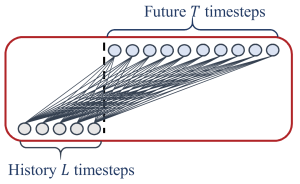
The core architecture of the DLinear and NLinear models is a single linear layer, with weights that map the input sequence directly to the output predictions. This design enables the models to generate predictions for all time steps in parallel rather than sequentially, which is known as a direct multi-step process (DMS).
Both the input and prediction window lengths are adjustable parameters that can be configured before training a model, enabling flexibility in selecting historical data ranges and forecasting horizons.

What differentiates these two models are the different types of pre-processing methods applied to the input sequence before it passes through the linear layer.
In the DLinear, the input sequence is decomposed, as follows:
- A moving average kernel is applied to the time series to extract the trend component. By subtracting the trend from the input sequence, we get the seasonality component
- Each of these components is passed through its own single linear layer
- The outputs from these separate layers are summed together
- This results in the final set of predictions
In the NLinear, the input sequence is normalised, as follows:
- The last value in the sequence is subtracted from the input
- This shifts the input values down, which are then passed through the linear layer
- The subtracted value is added back to the output sequence
- This results in the final set of predictions
The DLinear model is better suited for predicting the direction of prices in a time series, because of its ability to decompose the data into trend and seasonality components.
In contrast, the NLinear model excels when there are differing distributions of returns between the training and testing input time series due to its normalisation feature.
Transformer-based Architectures
Transformer models have achieved superior performance on natural language processing and generative tasks. Recently, they have become a focal point in time-series forecasting research due to their ability to model long-term dependencies in data.
Thanks to the effectiveness of their novel multi-head self-attention mechanism, these models can process sequences in parallel across many GPUs, rather than sequentially as was the case for RNNs and LSTMs.
The TFB, a comprehensive time series forecasting benchmark competition [2], tested various AI models, including the transformer models: Autoformer, FEDformer, and Informer, on time-series data spanning a wide range of domains.
In our study, we chose to compare the linear models to these state-of-the-art transformers, which are adaptations designed to improve upon the vanilla transformer. Here’s a breakdown of the innovations introduced in each model:
- Autoformer: Decomposes the input into trend and seasonality components to better model market drift
- FEDformer: Applies frequency transforms, such as Fourier, wavelet to better extract periodic movement
- Informer: Speed up model computation by reducing the time complexity of the self-attention mechanism from
O(L^2)toO(L log L)
Model Comparison
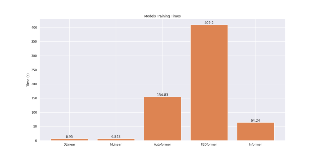
Shown below are the training times for all models, trained on an NVIDIA A10 GPU using the same input dataset and identical initial hyperparameters:

We can see that the linear models require significantly less training time, just a few seconds, compared to the transformer models, which can take over 6 minutes, as observed by the training time for the FEDformer.
Stylised Facts
Stylised facts are statistical metrics commonly observed in various financial time series data [3]. These properties are well-regarded amongst the finance research community as they capture real-world behaviour of asset prices and market movements.
Traditional machine learning evaluation methods, such as mean squared error (MSE), are not well-suited for forecasting over long time horizons, as they do not adequately account for the right amount of drift, volatility, or trading behaviour during sudden market crashes.
However, stylised facts are not widely used within the research literature we reviewed, as many papers resort to using MSE, RMSE, and MAE to evaluate model performance in their results sections. We encourage greater adoption of these metrics in the context of financial market data.
Therefore, we compared the performance of linear and transformer models using the following set of statistical metrics and stylised facts:
Statistical Metrics:
– Drift: Mean of percentage returns
– Volatility: Standard deviation
Stylised Facts:
– Volatility Clustering: Autocorrelation of squared log returns
– Heavy Tails: Distribution of log returns and computing the kurtosis to determine the tailed-ness of the distribution
– Intermittency: Fano Factors on log returns anomalies
During our analysis, we found that all models produced predictions that reflected market behaviour. This was evident in the stylised facts as follows:
- Decay in autocorrelation (volatility clustering)
- Kurtosis values greater than zero in the log returns distributions (heavy tails)
- Fano factors greater than 1.0 in the log returns anomalies (intermittency)
Limitations
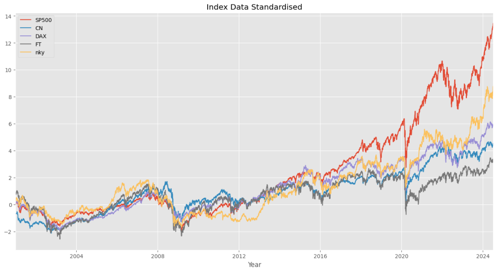
We faced a challenge while working with our dataset of index fund prices. The prices of each index fund were in dollars, but the values varied in scale due to the global nature of these markets. For example, the Japanese NIKKEI had prices over $10,000, whereas the S&P500 typically had prices in the low thousands.
We chose to standardise the prices using the z-score, which involves centering the mean of the values around zero and ensuring the standard deviation was around 1.0, before training the models on the data. Shown below are the standardised prices across the different indexes:

We trained the linear and transformer models using the same default hyperparameters as those in the original paper and TFB benchmark competition. However, there were some issues with the predictions from the linear models. In many batches of test data, the predicted values for the very first time step happened to be quite far from the final value in the input sequence. This had an impact on the results of certain stylised facts, such as volatility and volatility clustering.
We considered dropping the initial predicted value and recalculating the stylised facts on the rest of the predictions. Alternatively, we could also find a more optimal set of hyperparameters to retrain the models, potentially eliminating the sudden price swing.
Nevertheless, these linear models are very quick to train and deploy. As our results have confirmed that they outperform the more complex transformers, we believe that they are an ideal choice for long-term time-series forecasting. We would also like to encourage further research to explore other extensions of the vanilla linear model.